by Jantine Broek
Statistical Inference & Reproducibility
Part II: Frequentist vs Bayesian statistics
In the previous post, I started out with an explanation of general statistical inference and how a sample distribution relates to the population distribution and its parameters. Important to remember is the difference between a parameter and a statistic and that the conclusion of a statistical inference is a statistical proposition. Here, I continue with an explanation of the two types of statistical inferences: Frequentist and Bayesian inference. To get a better understanding of these two approaches, I will first discuss the concept of the likelihood function.
The likelihood function summarizes the data’s evidence about the unknown parameters and is used to generate estimators. The likelihood function is a function of a parameter and assumes the data, which means that it can be used only after data is available to describe the function of a parameter. Also, the likelihood is not a probability density function (pdf), as the pdf is a function of the data and assumes a parameter. The likelihood function plays a role in the different assumptions made for statistical inference between the Frequentist and Bayesian inference.
Frequentist inference
The Frequentist inference is the type of inference you would have learned while you were at school. This type of inference draws conclusions from sample data by justifying how it performs in infinitely many replications of the same hypothetical re-generation of the data. This interpretation of probability (as in p-values or confidence levels) is the long-run proportion of times in an infinite sequence of repetitions of the same experiment that some event will happen (like “null process generates test statistic as extreme or more extreme” for p-values, and “interval covers true parameter value” for confidence levels). Due to this infinite sequence of repetitions, the probability will approach a value which approximates a “fixed” population parameter. An example of a repeatable event would be drawing a certain hand of cards in a game of poker. When we say that an outcome has a probability of p of occurring, it means that if we would repeat the event, like draw another hand of cards, infinitely many times, then the proportion p of the repetitions would result in that outcome. As the probability is based on the frequency of an event occurring, the conclusion from the data is saying that you prove the null hypothesis with a given (high) probability.
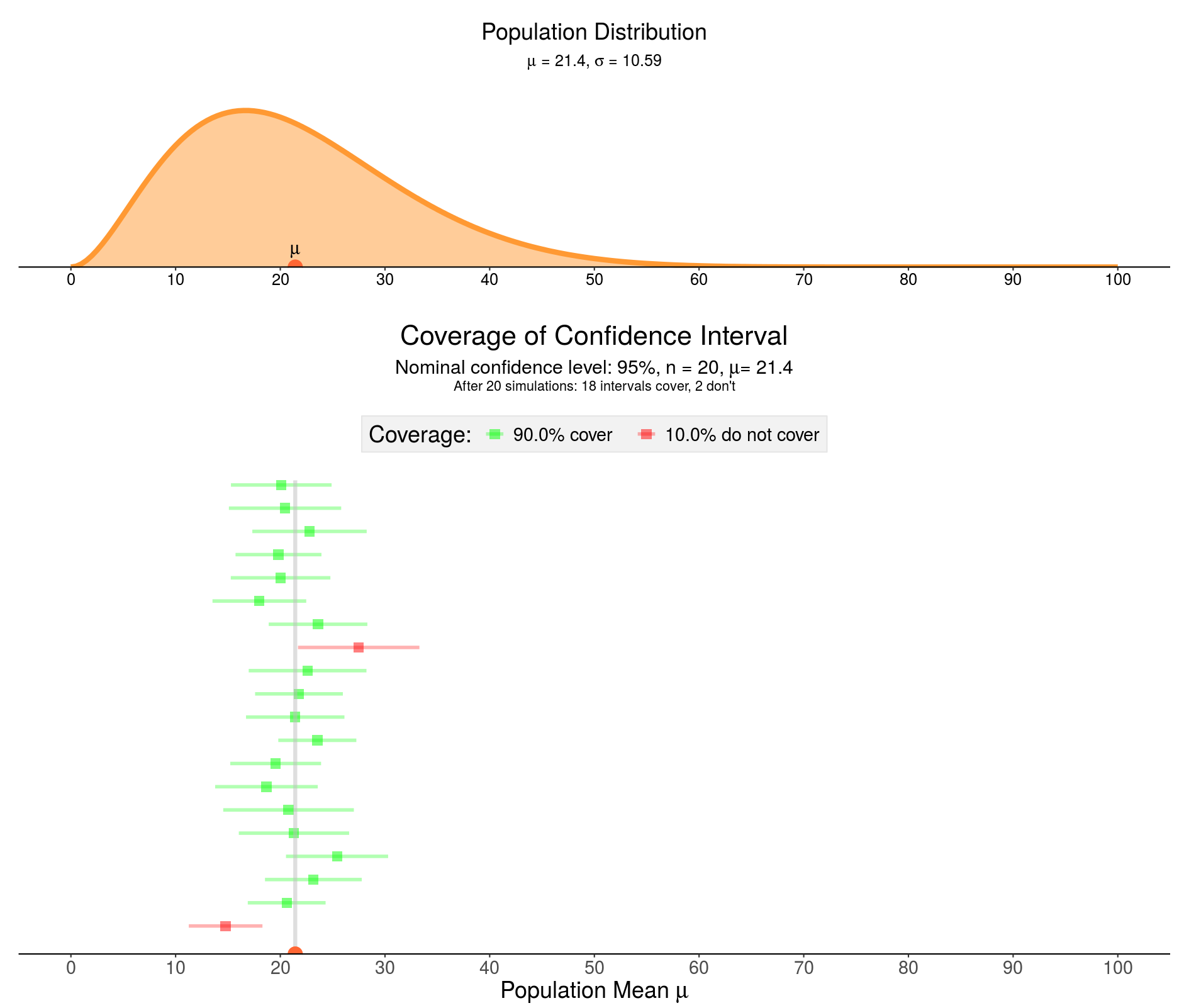
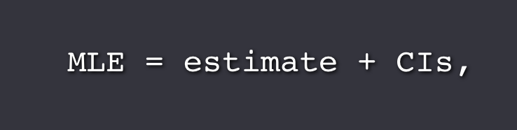
The uncertainty about the estimated parameter is captured by a range of values that include the true value of the unknown parameter with some minimum probability. This is the confidence interval (CI). The desired level of confidence is set by the researcher (and thus not determined by data). Most commonly, a CI of 95% is used. This means that out of every 100 experiments, at least 95 of the resulting CIs will be expected to include the true value of the parameter (see figure above). In Frequentist inference, the maximum likelihood estimate (MLE) method is often used to estimate a population parameter. In the MLE method, the population ‘estimator' value is set to the value that maximizes the likelihood function. This is analogue to choosing the parameter value for which the probability of the observed data set is maximized. Altogether, we can say that
Bayesian inference
We saw that, in order to infer something using the Frequentist approach, we relate directly to the rates at which events occur, or, in other words, the proportion of times something happens in a hypothetical infinite series of replications. For example, when we deal with repeatable events, such as coin flips or drawing a certain hand of cards in a game of poker, the outcome has a probability p of occurring. This means that if we repeated the experiment infinitely many times, then the proportion p of the repetitions would result in that outcome. However, this reasoning is getting problematic in situations that are not repeatable. For example, what if you would like to know the probability that the moon was once part of the earth. There is no way to make the Big Bang happen multiple times to test this probability. Therefore, we use the probability to represent a degree of belief, with 1 indicating absolute certainty, and 0 indicating absolute uncertainty. This latter probability that relates to qualitative levels of certainty, or belief, is known as Bayesian inference.
The Bayesian view is not the total opposite of the Frequentist view as it includes the notion of frequency, in addition to these unrepeatable events. The main difference between Frequentists and Bayesian inference is how you interpret what probability is and consequently how you treat the parameters. Instead of using the MLE as the best estimate for the parameters that indicates the probability of an event, the Bayesian approach uses the maximum a posteriori probability (MAP) to obtain a point estimate. The MAP is closely related to the MLE but it uses a penalty. This penalty is a prior distribution that quantifies the additional information available through prior knowledge of a related event, and is said to encompass belief. The distribution of the parameter is then defined on existing observations, saying "what is the probability of a given parameter value, given the data?"
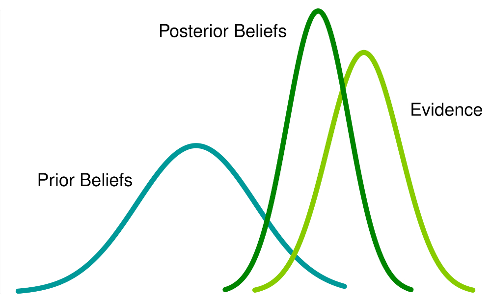
In both the Bayesian and Frequentist paradigms, the likelihood function plays a central role. However, the manner in which this is used is fundamentally different in the two approaches. In the Frequentist setting, the parameter is considered to be a fixed parameter, whose value is determined by using an MLE with a CI that considers the distribution of all possible data sets. This leads to either a "true or false" conclusion for a significance test. By contrast, from the Bayesian viewpoint, there is only a single data set (namely the one that is actually observed), and we assume that a prior distribution exists over the parameter that allows us to treat the parameter as a random variable. With these assumptions, we calculate the posterior distribution over the population parameter using the Bayes’ theorem, which says that the posterior is proportional to the product of the likelihood and prior, or

Therefore, the posterior probability is the probability of a parameter given the data and is analogous to a penalized likelihood where the penalty comes from an assumption on what possible parameter values should look like, which is given by the prior. Now, the uncertainty in the parameters is expressed through a posterior probability distribution over the parameter and the MAP estimates the parameter as the mode of the posterior distribution of the random variable.
In this second part of the blog “Statistical Inference and Reproducibility” I focused on the concepts of the two main statistical inference methods: Frequentist inference and Bayesian inference. The difference in concept of the two inferences is that the Frequentist probability is the proportion of times something happens in a hypothetical infinite series of replications, while the Bayesian probability represents the degree of belief. In the next post, I will discuss how proper usage of either type of statistical inference contribute to reproducibility, and that reporting the decisions you make in your statistical inference method are important for transparency and reproducibility of your statistical claim. In addition, I will discuss further strategies to increase the reproducibility in science.